OCR Text |
Show accordingly. As a result, prices might rise more than theory would indicate. FULL COST FEE ( PRICING SCHEMES) When the fee is to cover the cost of the product or service and not just be a percentage additional to the base price, more general micro economic theory is applicable. When the structure, goals, and management of a monopoly water supply system are analyzed, the theory suggests three broad strategies that might be used in relating price to costs of production. These strategies are marginal cost pricing, average cost pricing, and monopoly pricing. Although the user fees ( excise tax) considered in this study for generating state water development funds do not necessarily relate price to costs at the state level, it is useful to examine pricing policies in designing fee structures and establishing fee levels. Local organizations- mutual irrigation companies, municipalities, etc.- that have a state water fee imposed upon them can be expected to distribute this tax burden to their shareholders or customers. The effects of this distribution will depend to some extent on the pricing strategy a local unit employs. The state imposed fee may be considered in effect as an element of operating cost to these local organizations. Marginal and Average Cost Pricing Marginal cost pricing is the policy most conducive to the efficient use of resources. This policy sets the price at a level at which the marginal costs and benefits are equal. In other words, the user is charged a price for a resource that is equal to the incremental ( marginal) cost of production. In Figure 1 marginal cost is represented by curve MC, average cost is represented by curve AC, and demand is represented by line D. The most efficient price is located where the MC curve intersects the D curve ( Pe). When the price is set below marginal costs ( Pj) resources will be overused ( Qj). Alternatively, if prices are set above marginal costs ( P2), resources will be underused ( Q2). At price Pj the costs of producing quantity Q^ far exceed the price and result in a loss. At price P£, the price far exceeds the cost of producing quantity Q2. Only at Pe are the costs and revenues equated. Costs, however, do not always follow the pattern shown on Figure 1 in which marginal costs are increasing where they cross the demand curve. Municipal services are frequently thought to be decreasing cost industries ( each additional unit up to the total demand costs less to produce than the previous unit). In this case, pricing at marginal cost will fail to cover the costs of production ( Hoggan and Asplund, 1974), competing industries will be forced out of business, and the remaining monopoly will then be able to raise its prices to more than cover its costs. In Figure 2, AC represents the average cost of producing a commodity and includes a " fair" rate of return on the capital investment. MC represents the marginal cost of producing an additional unit, and D represents the demand of the commodity at any given price. Typically, the regulated price for a monopoly ( a decreasing cost industry) allows costs to be recovered, along with a " fair" return on investment. This is referred to as average cost pricing. At Pc, in Figure 2, the firm is covering costs as well as earning a fair rate of return on its investment. The determination of average cost is relatively easy, and given that costs are clearly specified, this approach is straight forward and considered equitable politically. However, if the price is set at the most economically efficient price Pe, the firm operates at a loss equal to the rectangle PjGHPe, and a subsidy would be required to maintain production. Either efficient pricing is sacrificed or the utility is subsidized. Price 02 Qe Ql Quantity Figure 1. Marginal cost pricing. Price c Pi P„ r * s?\ X/^ MC __________________ Ql Q2 Figure 2. Decreasing cost industry. Quanti ty 10 |