| Title |
Fuel Preheat as NOx Abatement Strategy for Oxygen Enriched Turbulent Diffusion Flames |
| Creator |
Amin, E. M.; Pourkashanian, Mohamed; Richardson, A. P.; Williams, Alan; Yap, L. T.; Yetter, R. A. |
| Publisher |
University of Utah |
| Date |
1994 |
| Spatial Coverage |
presented at Maui, Hawaii |
| Abstract |
The high thermal efficiencies achievable in industrial furnaces through oxygen enrichment has attracted much interest. As a result oxygen-enrichment techniques are used in various processes such as glass melting. ferrous as well as non-ferrous melting, cement production lime production. etc. With the higher temperatures and the availability of oxygen, generally increased emissions of NOx have to be tolerated. In this study measurements in a laboratory scale oxygen enriched turbulent diffusion flames of preheated methane are presented. An axisymmetric burner with coflowing oxygen enriched air is used which employs direct electrical heating of the methane. Experimental techniques included the measurement of the radiant fluxes from the flame using pyrometry, on-line gas analysis for combustion products and a laser extinction technique for the measurement of soot concentration. The flow field was computed using the k-8 with two step global reaction scheme. A simplified mechanistic model for soot formation is used. The model for soot and thermal NO was based on the laminar flamelet model. The fluctuations in the mixture fraction was a clipped Gaussian pdf. Results have shown that fuel preheating can locally reduce the temperature through enhanced soot formation. This results in a reduction in the EINOx emission as a result of reduced thermal NO formation. |
| Type |
Text |
| Format |
application/pdf |
| Language |
eng |
| Rights |
This material may be protected by copyright. Permission required for use in any form. For further information please contact the American Flame Research Committee. |
| Conversion Specifications |
Original scanned with Canon EOS-1Ds Mark II, 16.7 megapixel digital camera and saved as 400 ppi uncompressed TIFF, 16 bit depth. |
| Scanning Technician |
Cliodhna Davis |
| ARK |
ark:/87278/s6tq644x |
| Setname |
uu_afrc |
| ID |
9480 |
| Reference URL |
https://collections.lib.utah.edu/ark:/87278/s6tq644x |