| OCR Text |
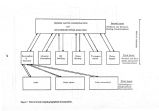
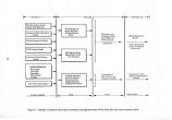
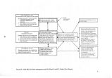
Show The model will be developed to predict seasonal trends, rather than short term changes, within the lake system. Under this time resolution it is anticipated that distributions in the lake will approach steady- state conditions and that the rate change in concentrations with respect to time goes to zero. If input flow and current patterns are those averaged over the season of interest, Equations 1 and 2 are further simplified to a system having constant coefficients. An efficient solution algorithm will be based on a stepwise procedure ( Grenney and Bella, 1971) which incorporates both numerical and closed- solution techniques. Besides being able to predict the effects of upstream ( watershed) changes on the hydrologic and. salinity aspects of the lake, the model will be capable of monitoring important water quality constituents, including: Ammonia - nitrogen may be a limiting factor in micro- organism growth Phosphorous - important in ecological systems and many leach out of bottom sediments Biological oxygen demand ( BOD) - an important parameter in state water quality monitoring and an indicator of pollution levels Coliforn bacteria - an important parameter in state water quality monitoring and an indicator of the presence of disease causing bacteria Temperature - an important parameter in determining the potential biological activity Dissolved oxygen ( DO) - an important parameter in state water quality monitoring and important to the healthy state of important living organisms, such as brine shrimp Model Verification Computer synthesis The basic premise of the approach discussed by this report is the representation of the Great Salt Lake and its surrounding basin by a hierarchy of mathematical models. The physical component of the overall system will be represented by describing and simulating the real physical system of the lake as accurately as is both possible and feasible. In particular, the coupling relationships among the various systems inputs, outputs, exogenous variables, and other decision variables are related and accounted for in the model. A computer model of a water resource system is produced by programming on a computer the mathematical relationships and logic functions of the system model. The model does not directly simulate the real physical system, but is analogous to the prototype because both systems are described by the same mathematical relationships. A mathematical function which describes a basic process, such as evapotranspiration, is applicable to many different hydrologic systems. The simulation program developed for the computer incorporates general equations of the various basic processes which occur within the system. The computer model, therefore, is free of the geometric restrictions which are encountered in simulation by means of network analyzers and physical models. The model is applied to a particular prototype system by establishing, through a verification procedure ( sometimes called validation or parameter identification), appropriate values for the " constants" of the equations required by the system. Model calibration and testing A general model is applied to a particular system ( often referred to as the prototype) through a verification procedure whereby the values of certain model parameters are established for that particular system. Verification of a simulation model is performed in two steps, namely, calibration ( parameter identification), and testing of the model. Data from the prototype system are required in both phases of the verification process. Model calibration involves adjustment of the model parameters until a close fit is achieved between the model output and the corresponding observed output of the prototype system. It therefore follows that the accuracy of the model cannot exceed that provided by the historical data from the prototype system. Evaluation of the model parameters can follow any desired pattern, whether it be random or specified. Model Operation The model is, of course, operated during the verification procedure, and at this time comparisons are made to test the ability of the model to represent the system or subsystem of the real world. It is very possible that these tests will indicate that some adjustments are necessary, either in the need of more data on which the model is based, or in the structure of the model itself. The various options associated with this looping, or " feedback" procedure are indicated by the flow path labeled " compromises" on the diagram of Figure 4. When suitable model verification has been achieved, the model is ready for use as a technique for investigating the response of the system to various input conditions and management alternatives which might be imposed. In the case of this study, each component or subsystem model will be capable of operating either independently or in conjunction with the models of other components of the total system depicted by Figure 7. 42 |


